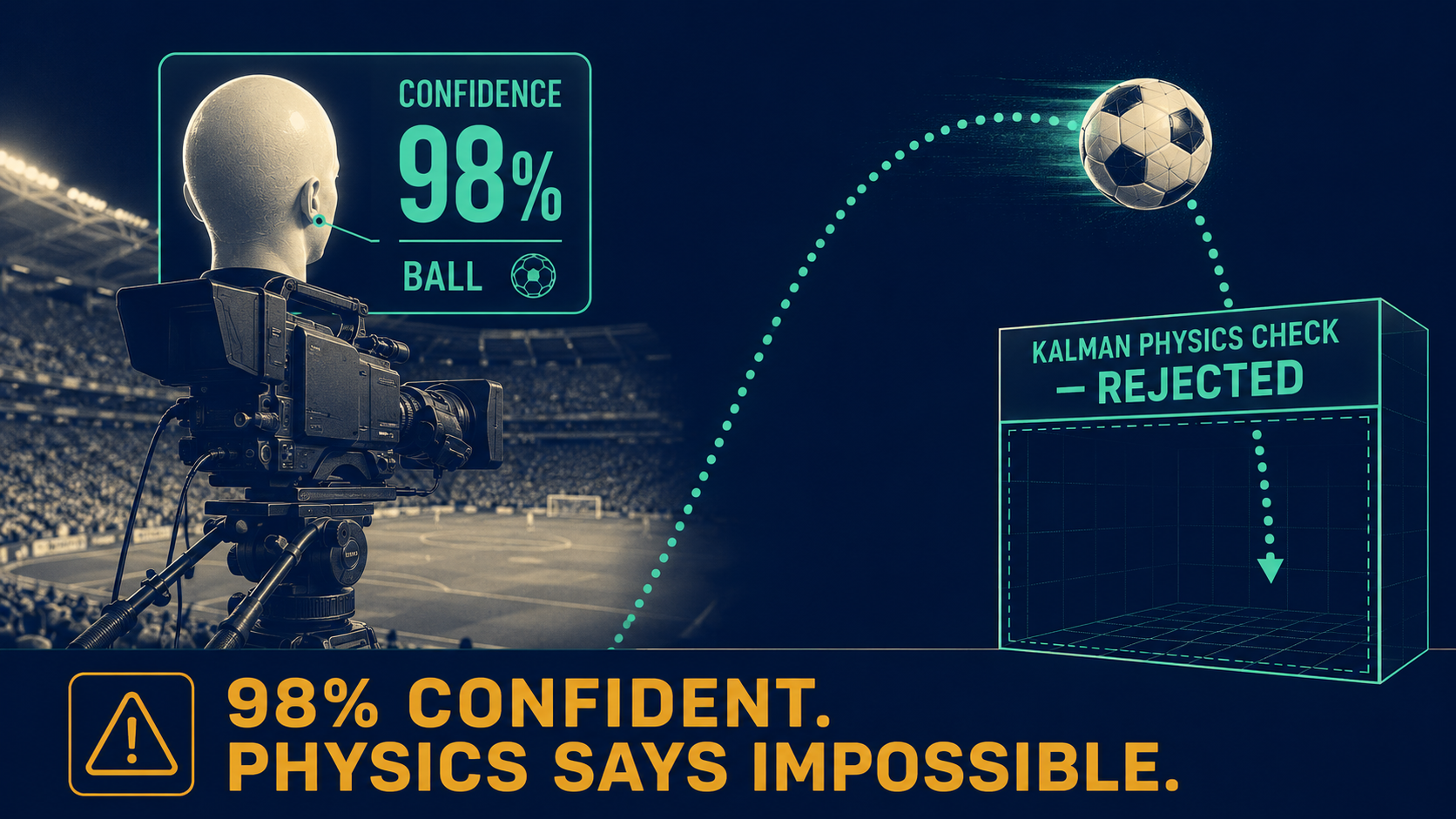
The standard response to a false positive in computer vision is to raise the confidence threshold. That also explains why false positives in high-stakes deployments — sports tracking, semiconductor inspection, manufacturing quality control — tend to plateau once standard calibration approaches have been exhausted. Confidence thresholds operate on visual pattern scores and have no model of what's physically possible. The automated camera system that tracked a linesman's bald head for an entire match at Inverness Caledonian Thistle in 2020 was doing so at 98% confidence — higher than many correct ball detections. Raising the threshold to 99% wouldn't have changed the outcome. Under stadium floodlights, the specular highlights on the linesman's head produced pixel gradients statistically indistinguishable from a white soccer ball. What would have changed the outcome: a physics check. A ball doesn't move at constant 1.7-meter height at 3 mph while remaining attached to a vertical cylindrical object. The detector had no way to know that. A Kalman filter does.
We've studied this failure mode across broadcast sports, semiconductor fabrication, and discrete manufacturing. The root cause is consistent: detectors find visual patterns. They don't understand physics. Until the pipeline includes a physics layer that rejects physically impossible detections, false positive rates remain a function of the training data distribution rather than a function of what can actually happen.
Our work on physics-constrained computer vision addresses this at inference — where the false positives actually occur — rather than at training time.
When the Nuisance Rate Is the Problem, Not the Detection Rate
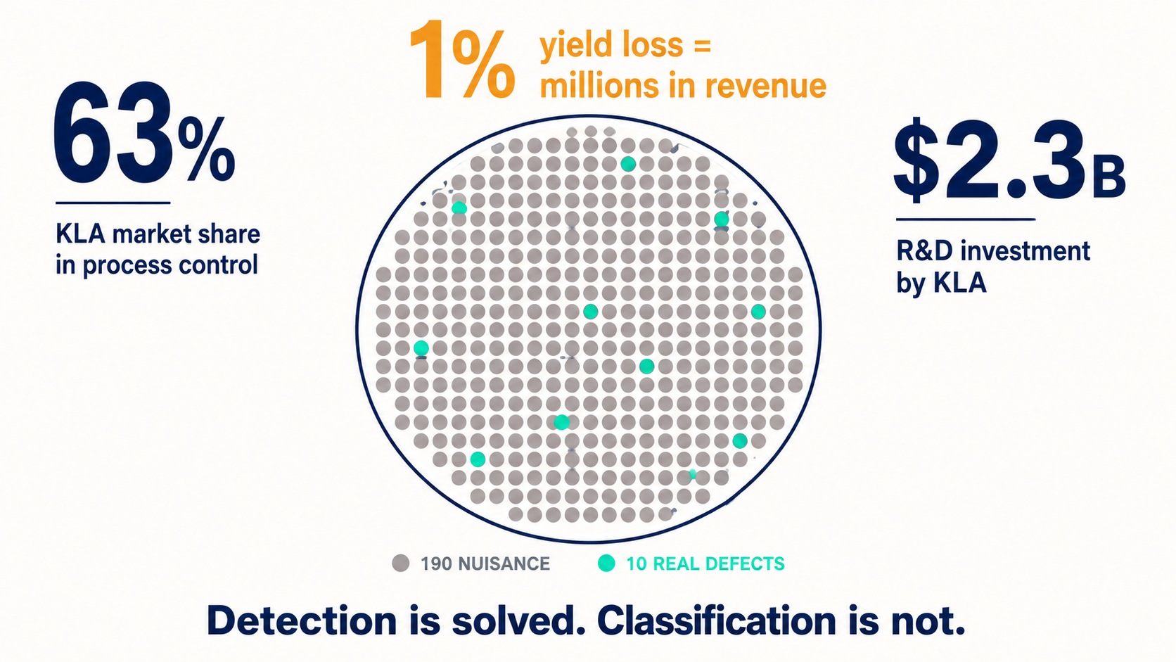
KLA Corporation holds 63% of the semiconductor process control market, and their 2900 Series broadband platform detects yield-relevant defects at features as small as 10nm — the output of $2.3 billion in R&D investment. Detection capability at that scale is not the bottleneck.
The nuisance defect problem is. At advanced process nodes, a single broadband scan flags thousands of anomalies per wafer. The majority are surface artifacts, dust particles, or pattern noise that won't affect yield. Each requires classification. Each classification routed to human review burns engineer time at the same rate whether the defect is real or not, and yield-relevant defects can get missed in the volume.
A 1% yield loss at advanced nodes translates to millions in lost revenue. Individual wafer cost at leading-edge processes can exceed tens of thousands of dollars. The nuisance defect problem isn't primarily a quality issue — it's an engineering economics problem.
Classifiers trained on historical defect libraries have no internal model of how light physically interacts with a pit versus a surface stain versus process residue. They've learned correlations that held for the old process node. When a fab transitions to a new one, the materials scatter light differently, and the learned correlations don't transfer. The nuisance rate spikes. The available remediation — retrain, or raise the acceptance threshold — either takes time or trades nuisance reduction against missed real defects.
Physics-based features capture what the imaging physics actually encodes: parallax behavior across inspection angles (a real pit creates a depth-dependent shift; a surface particle doesn't), material reflectance profiles tied to known composition, topographic scattering patterns that separate surface from subsurface anomalies. These features hold across node transitions because the physics of light interaction with a geometric structure doesn't change with the process chemistry. On the nuisance defect triage logs we've reviewed after node transitions, the pattern is consistent: the confusion matrix degrades on purely visual features and holds on physics-grounded ones.
Silent Drift Doesn't Announce Itself
The semiconductor nuisance problem is at least visible — engineers see the triage queue growing. On manufacturing production lines, the equivalent problem is structurally silent.
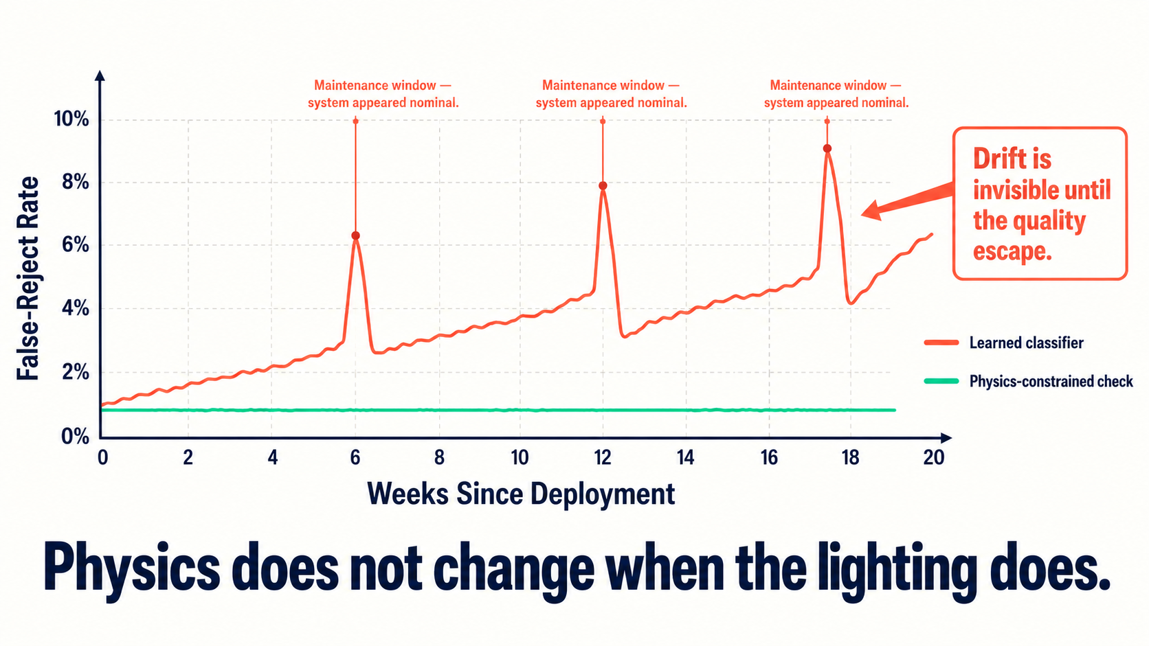
On lines using AI-based quality control, there are no real-time ground-truth labels during live production. A lighting angle shifts after a maintenance window. A lens hazes over weeks. A fixture wears. False-reject rates accumulate quietly — more good parts pulled for rework — or false-accept rates creep upward as defects escape into finished inventory. By the time a quality escape surfaces, it's already triggered broad containment and re-inspection. The cost of poor quality runs approximately 20% of total sales for average manufacturers. Intel has documented $2 million annually in AI vision inspection savings — starting from a waste floor that was already large.
Physics constraints respond differently to environmental drift than learned classifiers do. The physical properties of a correctly manufactured part — its geometry, its surface reflectance, its material composition — don't change when the lighting shifts. A physics-informed check asks whether the observed image is consistent with the known material and geometry model, not whether it "looks like" a good part compared to historical training images. Production-line trend data across deployments shows that physics-constrained checks maintain stable rejection rates through maintenance windows and environmental variation in ways that purely learned classifiers don't.
Why Confidence Tuning Hits a Ceiling
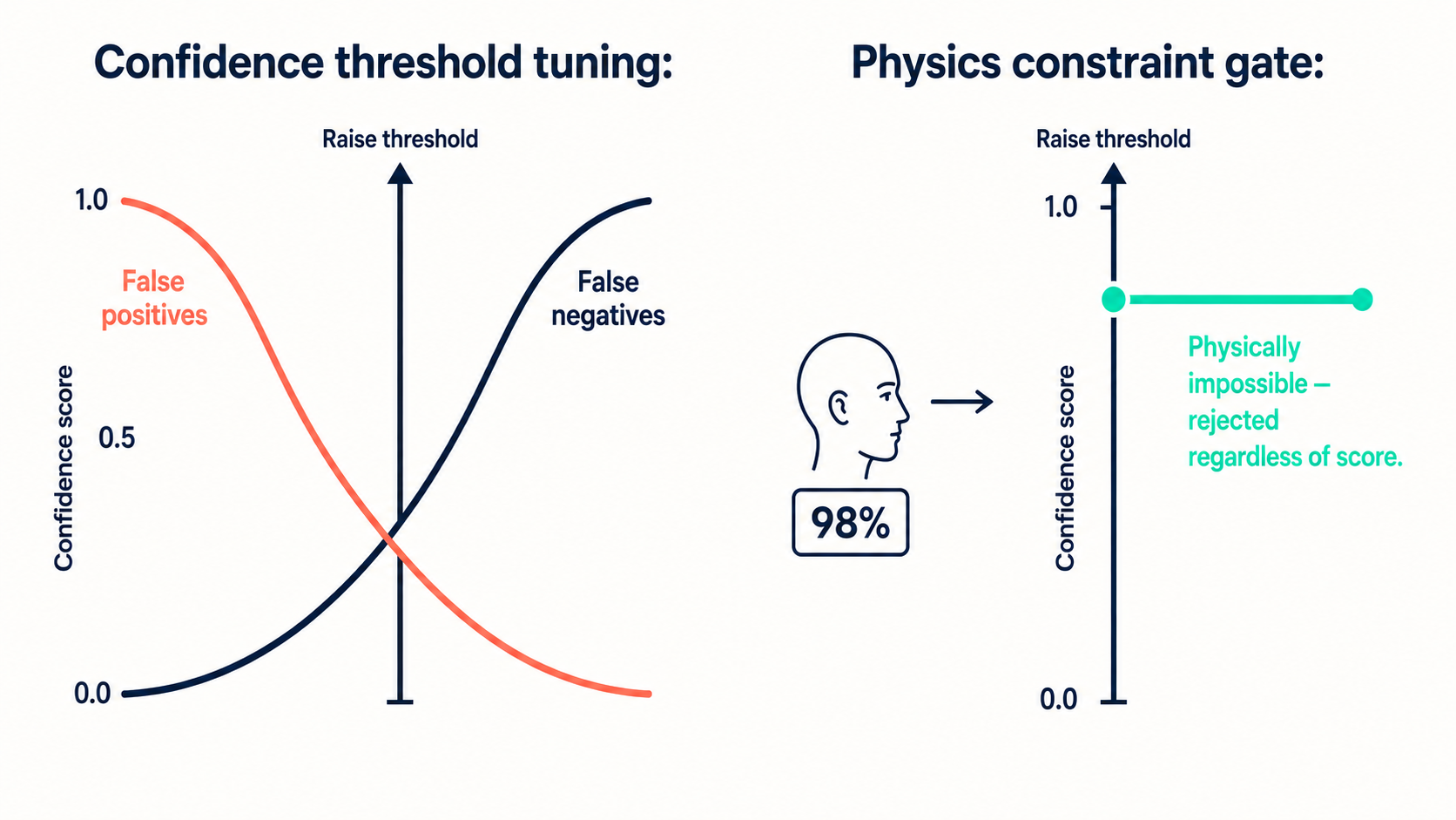
The standard false-positive reduction sequence — more diverse training data, higher thresholds, ensemble methods, calibration adjustments — produces real improvements up to a point. Autoencoders applied as post-processing filters have shown 22.5–87.2% reductions in false positives in research settings. The ceiling appears when the source of false positives is a genuine visual ambiguity: the linesman's head really does look like the ball under those lighting conditions. No calibration technique closes that gap because the data-generating process produces genuinely ambiguous examples.
Physics constraints work orthogonally to confidence thresholds. They don't raise the bar — they add a perpendicular check. A detection that's physically impossible is rejected regardless of the detector's visual confidence. A detection that's physically plausible passes even if the visual confidence is moderate.
The most common case is temporal consistency across frames: the same tracked object should follow a physically plausible trajectory. A Kalman filter addresses this by maintaining a predicted state — position, velocity, trajectory — and rejecting candidates that fall outside the prediction boundary regardless of visual confidence. That handles the bald head problem. Where Kalman handles temporal consistency, optical flow handles spatial consistency: does this detection move the way everything around it is moving, or is it an isolated anomaly that doesn't cohere with the scene? A detection that can't be explained by the local motion field gets flagged as physically anomalous. The third check applies where two synchronized cameras are available — epipolar geometry constrains where a real 3D object can appear in both views simultaneously. A surface artifact that reads as a defect from one inspection angle won't produce the corresponding parallax in the second view; it dissolves, while a real subsurface defect holds its position in both.
None of these checks require retraining. None of them drift with data distribution. They add between 2 and 8 milliseconds of processing per frame and sit between the detector and the action system.
What the Vendors Have Solved and What They Haven't
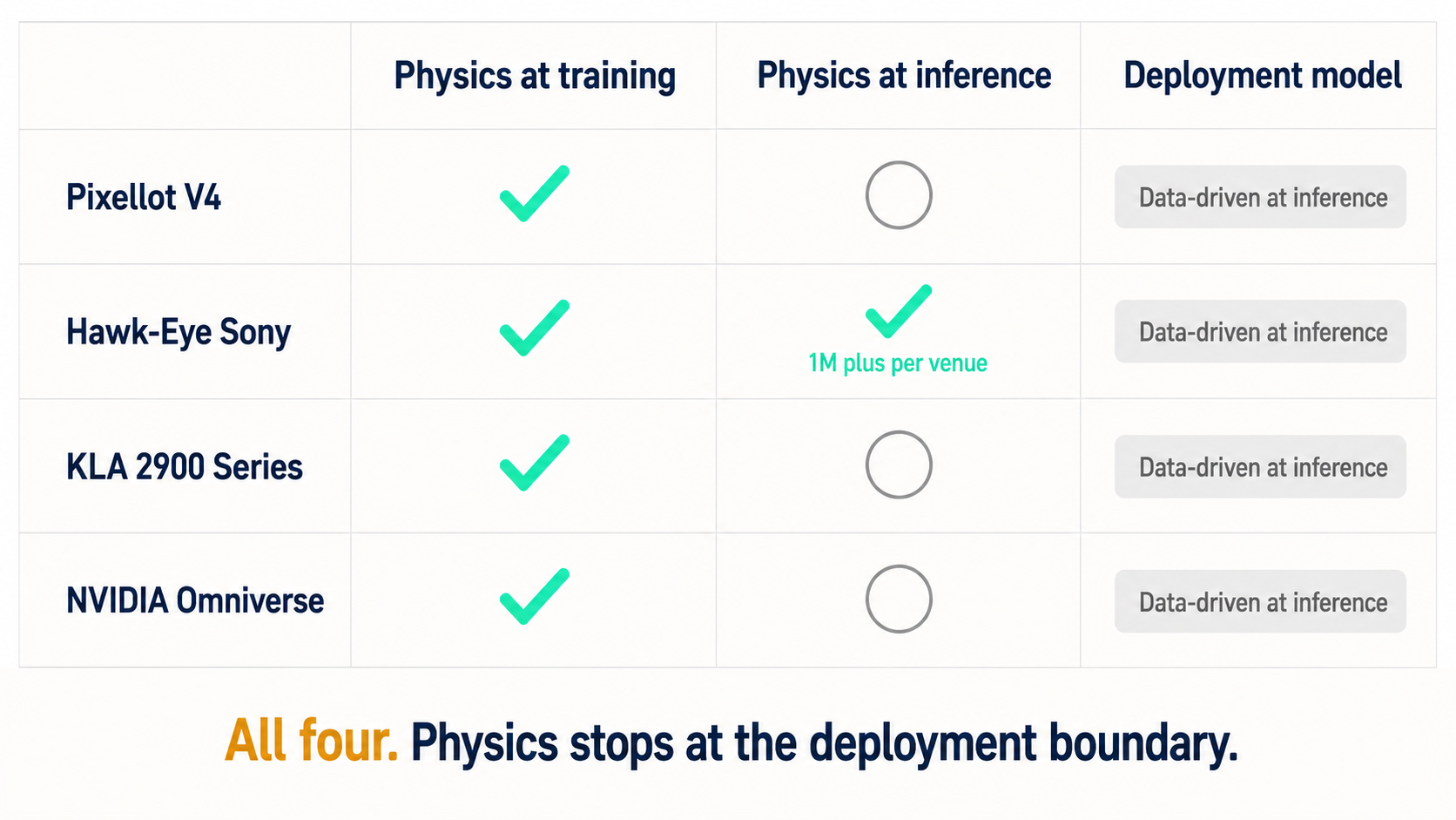
Pixellot's V4 multi-hypothesis tracking addressed the bald-head class of errors for professional broadcast. Hawk-Eye, now a Sony company, deploys multi-camera triangulation tracking 29 skeletal points per player — running in NFL stadiums with six 8K cameras per venue in the 2025 season, and across all nine ATP Masters 1000 events in 2026. These are real advances. The gap in the Pixellot architecture is that multi-hypothesis tracking is post-hoc disambiguation between candidates — the system still has no kinematic model of what's impossible, and new failure modes (jersey OCR under motion blur, offside projection on non-flat pitch surfaces) persist with the same root cause. Hawk-Eye's multi-camera geometric constraints do represent physics integration, but at $1 million or more per venue, that infrastructure scales to World Cup venues, not to the 40,000+ clubs using Veo cameras across 100 countries.
KLA's $2.3 billion R&D investment and MCAT iDO 3.0 machine learning layer aim at the nuisance defect problem. NVIDIA's Omniverse and Cosmos platforms use physically accurate rendering to generate synthetic training data. The pattern across all of these: physics enters at the development stage and stops at the deployment boundary.
The gap isn't whether physics is present in the development pipeline. It's whether physics is present at inference — where the live production footage is processed and the false positives actually occur.
That specific gap is where the work we've described at physics-constrained computer vision operates.
What August 2026 Changes for Auditable CV
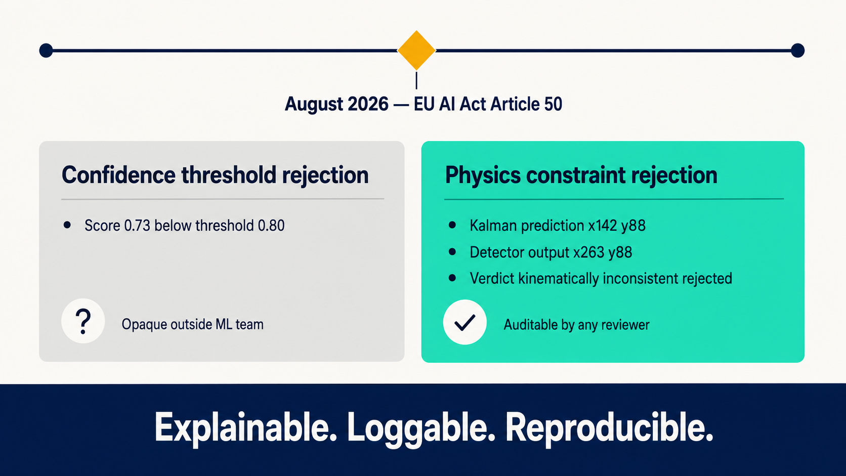
For CV systems making decisions that affect people — access control, workplace monitoring, sports officiating — the EU AI Act's transparency obligations under Article 50 take full effect in August 2026. Physics-constrained rejection decisions have a structural compliance advantage: they're deterministic and auditable. A detection was rejected because the Kalman filter's predicted state was kinematically inconsistent with what the detector reported. That's a reproducible, loggable reason, readable by a non-ML reviewer. A pure confidence-score threshold is not: it's opaque outside the team that set it.
The SoccerNet multi-object tracking benchmark is explicit about where the research gap sits. Tracking across dense player configurations, fast motion, and heavy occlusion is described in the benchmark's own documentation as "far from solved." No physics-aware tracking approach appears in the leading methods on the HOTA and DetA leaderboard columns — the benchmark tracks exactly the conditions where physics-naive systems produce the most irreducible errors.
The 95% That Never Ship
Industry data from 2025 puts the share of computer vision projects that never reach production at 95%. The failure modes are consistent: models built in controlled lab conditions break on the factory floor because ambient lighting changes, fixtures wear, and operators vary. Edge cases — scenarios rare in training data and common in production — account for the majority of engineering time, support cost, and liability exposure once a system is live.
More robustness testing and staged deployment are the right procedural responses. They don't change the underlying limitation: a neural network trained on controlled conditions has no knowledge of what's physically impossible. That knowledge has to be explicitly encoded.
If your team has a CV deployment where false positive rates have plateaued above operational threshold and standard calibration has reached its ceiling, we'd like to work through the architecture. The conversation on physics-constrained computer vision gets specific quickly — what the Kalman state model needs to represent, what the detector is already producing, where the physics model can be derived analytically versus where it needs calibration. The constraint layer is usually simpler to add than it appears from the outside, and its stability over time tends to be the most durable benefit.